
by Sylvain Artois on Jun 5, 2025
For the past few weeks, I’ve been working on a project to extract headlines from the press in order to generate “non-manipulable” trends, as an alternative to those found on social media where simply deploying an army of bots can create artificial trending topics. To create meaningful trends, we first need to be able to group different headlines by theme - this is the classic ML discipline of clustering. And to perform good clustering, we need the ability to evaluate and measure the relevance of our categorization.
I propose here to review the fundamentals, starting from an imaginary binary classifier that will allow us to establish the foundational metrics used to evaluate supervised ML algorithms, then expand to the evaluation of supervised NLP clustering. This detour through the basics - the binary classifier - is what I felt was missing in my understanding of clustering evaluation, something that took me time to find elsewhere, and therefore what I’m trying to offer here.
We’ll work with real data, simplified. This is more meaningful than abstract data.
On April 25th, 2025, we had these few headlines in the French press (id, title, imaginary probability from our non-existent binary classifier, ground-truth):
Traditionally, a binary classifier returns a float between 0 and 1, which can be interpreted as the probability of a data point belonging to one of two classes1.
Here, our imaginary binary classifier answers the question “Does the headline evoke the Israel/Hamas war?”
Four categories are used to evaluate an implementation2:
We can then count the cases for each category and construct a confusion matrix, which helps visualize the results:
| Prediction | |||
|---|---|---|---|
| Positive | Negative | ||
| Ground Truth | Positive | TP: [1,2,3] 3 |
FN: [5] 1 |
| Negative | FP: [4,7] 2 |
TN: [6] 1 |
|
From this foundation, two fundamental metrics can be calculated that underpin the evaluation of many supervised ML algorithms :
This can be read as: among all the headlines that the model identified as evoking the Israel/Hamas war, what proportion actually evokes it?
Here we have
Among the headlines that evoke the Israel/Hamas war, what proportion did the model actually detect?
Here we have
Wikipedia provides well-crafted diagrams that help visualize what precision and recall measure
Both metrics are evaluated together to avoid classic misunderstandings:
A unified metric was therefore created, the F1-score, which is the harmonic mean of precision and recall:
In our example, we have
The F1-Score is only high if both precision and recall are high, and collapses if either one is low.
sklearn provides implementations of precision, recall and F1 score.
By convention, in most ML implementations, inputs (features, data) are prefixed with X, and outputs with Y (target, labels). For an ML-newbie like me, this was confusing, so I’m clarifying even though I have no source…
import sklearn

y_true = [1,1,1,0,1,0,0]
y_pred = [1,1,1,1,0,0,1] # with a threshold at 0.9

print(sklearn.metrics.precision_score(y_true, y_pred)) # 0.6
print(sklearn.metrics.recall_score(y_true, y_pred)) # 0.75
print(sklearn.metrics.f1_score(y_true, y_pred)) # 0.6666666666666666So every morning I receive 700 headlines, and I want to group them to define trends. Let’s take our reduced dataset and try to cluster it manually:
Two things can be observed:
This is somewhat different from the traditional field of clustering where we seek to make data speak: let’s cite the popular k-means clustering algorithm, applied for example in marketing to segment a population (age, income, gender, …), where there are no labels, and thus the evaluation metrics are different (see silhouette score, Calinski–Harabasz index, Davies–Bouldin index).
The question is: how can TP/FP/TN/FN be calculated when naively we would rather want to answer, for such title, is the prediction of belonging to such cluster correct or not? A naive method might be used in very specific cases where we are certain that y_true and y_pred have exactly the same clusters, but in most cases, humans and machines will return different clusters, probably even a different number of clusters, so correspondence between each cluster would first need to be found.
Pair confusion matrix arising from two clusterings.
The pair confusion matrix computes a 2 by 2 similarity matrix between two clusterings by considering all pairs of samples and counting pairs that are assigned into the same or into different clusters under the true and predicted clusterings.
Considering a pair of samples that is clustered together a positive pair, then as in binary classification the count of true negatives is C00, false negatives is C10, true positives is C11, and false positives is C01.
This equivalence table can be constructed3:
| Category | Definition (by pair of points) |
|---|---|
| True Positive (TP) | Both points are in the same cluster, and should be |
| False Positive (FP) | Both points are in the same cluster, but shouldn’t be |
| False Negative (FN) | Both points are in different clusters, but should be together |
| True Negative (TN) | Both points are in different clusters, and should be |
Let’s add invented y_pred to our headlines dataset:
| Article | y_true | y_pred |
|---|---|---|
| Opinion. In Gaza, Netanyahu | Israel vs Hamas War, 1 | Israel vs Hamas War, 1 |
| Gaza: at least 50 Palestinians | Israel vs Hamas War, 1 | Israel vs Hamas War, 1 |
| ”Are we going to die tonight?” | Israel vs Hamas War, 1 | Israel vs Hamas War, 1 |
| ”B-52 or the one who loved Tolstoy” | Vietnam War Literature, 2 | Israel vs Hamas War, 1 |
| An Israeli singer calling to | Israel vs Hamas War, 1 | Israeli Pop Culture, 5 |
| Death of Pope Francis: why the | Death of Pope Francis, 3 | Death of Pope Francis, 3 |
| War in Ukraine: Russian general | War in Ukraine, 4 | Israel vs Hamas War, 1 |
Precision / recall / F1_score can now be calculated via sklearn’s pair_confusion_matrix:
from sklearn.metrics import pair_confusion_matrix

y_true = [1,1,1,2,1,3,4]
y_pred = [1,1,1,1,5,3,1]

tp, fp, fn, tn = pair_confusion_matrix(y_true, y_pred).ravel()

precision = tp / (tp + fp) if (tp + fp) > 0 else 0
recall = tp / (tp + fn) if (tp + fn) > 0 else 0
f1_pairwise = 2 * precision * recall / (precision + recall) if (precision + recall) > 0 else 0

print("== Pairwise Evaluation ==")
print(f"TP = {tp}, FP = {fp}, FN = {fn}, TN = {tn}")
print(f"Precision = {precision:.3f}")
print(f"Recall    = {recall:.3f}")
print(f"F1-score  = {f1_pairwise:.3f}")
The result obtained:
== Pairwise Evaluation ==
TP = 16, FP = 14, FN = 6, TN = 6
Precision = 0.533
Recall = 0.727
F1-score = 0.615The pairwise F1-score alone is insufficient, as it offers only a first estimation of coherence between two clusterings. But this approach remains partial: it evaluates pairs of points, without considering the structure of the clusters themselves. Two very different clusterings can result in the same pairwise F1-score if they preserve a sufficient number of correctly grouped pairs.
I’ve presented it for pedagogical purposes, to make the connection with the fundamental evaluation methods of a binary classifier.
I’m basing this on the chapter “Flat Clustering, Evaluation of clustering” from Introduction to Information Retrieval (2008), which I encountered often during my explorations.
I won’t try to paraphrase this or that source, and simply cite the scikit learn documentation, which is decidedly indispensable:
The Rand Index computes a similarity measure between two clusterings by considering all pairs of samples and counting pairs that are assigned in the same or different clusters in the predicted and true clusterings. The raw RI score is then “adjusted for chance” into the ARI score using the following scheme: The adjusted Rand index is thus ensured to have a value close to 0.0 for random labeling independently of the number of clusters and samples and exactly 1.0 when the clusterings are identical (up to a permutation). The adjusted Rand index is bounded below by -0.5 for especially discordant clusterings.
scikit-learn.org, adjusted_rand_score
I came across Permetrics on my journey, which offers implementations of various evaluation measures for ML algorithms, and well-crafted documentation, which I cite here to explain purity:
It measures the extent to which the clusters produced by a clustering algorithm match the true class labels of the data. Here’s how Purity is calculated:
- For each cluster, find the majority class label among the data points in that cluster.
- Sum up the sizes of the clusters that belong to the majority class label.
- Divide the sum by the total number of data points. The resulting value is the Purity score, which ranges from 0 to 1. A Purity score of 1 indicates a perfect clustering, where each cluster contains only data points from a single class. Purity is a simple and intuitive metric but has some limitations. It does not consider the actual structure or distribution of the data within the clusters and is sensitive to the number of clusters and class imbalance. Therefore, it may not be suitable for evaluating clustering algorithms in all scenarios.
permetrics.readthedocs.io, Purity Score
Here we start from information theory, where Shannon defines a measure, the Mutual information.
I’m afraid of saying something wrong by paraphrasing, so I’ll cite Wikipedia:
In […] information theory, the mutual information (MI) of two random variables is a measure of the mutual dependence between the two variables. More specifically, it quantifies the “amount of information” (in units such as shannons (bits), nats or hartleys) obtained about one random variable by observing the other random variable.
wikipedia.org, Mutual information
Then, once again, the scikit learn documentation should be read, which I cite:
Given the knowledge of the ground truth class assignments labels_true and our clustering algorithm assignments of the same samples labels_pred, the Mutual Information is a function that measures the agreement of the two assignments, ignoring permutations. Two different normalized versions of this measure are available, Normalized Mutual Information (NMI) and Adjusted Mutual Information (AMI). NMI is often used in the literature, while AMI was proposed more recently and is normalized against chance.
scikit-learn.org, Mutual Information based score
We’ve seen that Precision and Recall must be evaluated together to correctly assess an algorithm. Depending on whether we seek to penalize false positives (spam detector) or false negatives (diagnostic aid), the F1-score can be weighted:
We can use the F measure to penalize false negatives more strongly than false positives by selecting a value β > 1, thus giving more weight to recall
from Introduction to Information Retrieval, Evaluation of clustering
Many other metrics are possible, the field is vast, I’m only offering a humble introduction here. Measuring the performance of implementations is just the basics, both indispensable, but not always sufficient…
In ML Flow, artifacts can be added, here for example is a map of our clusters, which I always look at:
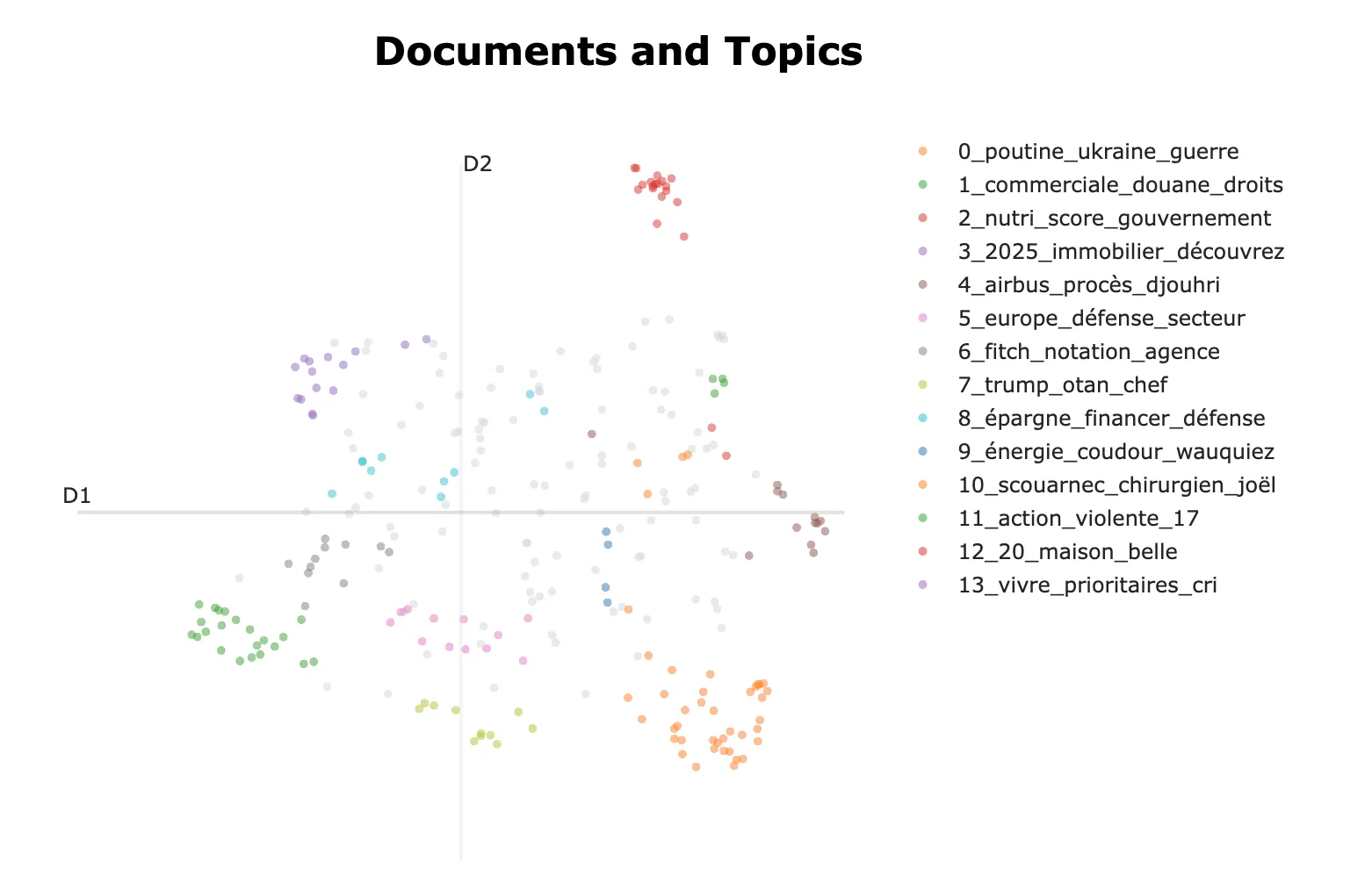
Working on a few well-mastered datasets, manually labeled, even if I introduce biases, allows me to “feel” naive metrics, for example, do my current parameters allow separating the “Le Scouarnec Trial” (horrible pedocriminal case) from the “Libyan Sarkozy Trial” (supposed financing of a French former president’s campaign by Gaddafi), which I think is essential to separate and which are yet often merged. A few metrics, good experiment tracking software, lots of graphs, and working on reduced and well-mastered datasets, this might be a key.
See the implementation via Keras proposed by François Chollet in Deep Learning with Python, 4.1 Classifying movie reviews: A binary classification example ↩
See Deep Learning, a visual approach by Andrew Glassner, Chapter 3, Measuring performance. ↩
Read Evaluation of clustering from Introduction to Information Retrieval, By Christopher D. Manning, Prabhakar Raghavan & Hinrich Schütze, 2008 ↩